Introduction

The Lamb weather type is a method of classifying synoptic weather pattern created by H.H. Lamb [Lamb, 1972]. It is based on the surface pressure values in and around the British Isles. The Lamb system classify the prevailing synoptic conditions into ten distinguished categories: eight directional categories (compass card), and two vorticity categories (cyclonic or anticyclonic). More recently, an objective scheme to classify the daily circulation according to the Lamb weather typing scheme was developed by Jenkinson and Collison [Jenkinson and Collison, 1977].

In section Methods, the methods of the calculation procedure are described. Sections Input and Output explain the input respectively the output of the Circulation Weather Types (CWT) tool.

Methods

The objective scheme uses daily grid-point mean sea level pressure data (see Fig. 1). The objective and the original subjective Lamb scheme have been compared by Jones et al. [1993]. Jenkins and Collinson extended the original Lamb weather types to 26. They added hybrid types of the pure direction and anti/cyclonic types.

Fig. 1 Location of the grid points over the British Isles used in the calculation of the Jenkinson flow and vorticity terms. Grid-point numbers are thosed used in the equations.

Using the grid-point numbers in Fig. 1 the wind-flow can characteristic by westerly flow, southerly flow, resultant flow, westerly shear vorticity, southerly shear vorticity an total shear vorcitity.

\[\begin{split}\begin{split} \text{W} &= \frac{1}{2}(12+13)-\frac{1}{2}(4+5) && \text{(westerly flow)} \\ \text{S} &= \frac{1}{cos(\text{lat})}\bigg[\frac{1}{4}(5+2\cdot9+13) - \frac{1}{4}(4+2\cdot8+12)\bigg] && \text{(southerly flow)} \\ \text{F} &= (\text{S}^2+\text{W}^2)^{\frac{1}{2}} && \text{(resultant flow)} \\ \end{split}\end{split}\]

\[\begin{split} \text{ZW} &= \frac{sin(\text{ lat})}{sin(\text{lat - 5})} \bigg[ \frac{1}{2}(15+16)-\frac{1}{2}(8+9)\bigg]- \frac{sin(\text{lat})}{sin(\text{lat + 5})} \bigg[ \frac{1}{2}(8+9)-\frac{1}{2}(1+2)\bigg]&& \end{split}\]

\[\begin{split} &&\text{(westerly shear vorcitiy)} \end{split}\]

\[\begin{split} \text{ZS} &= \frac{1}{2\cdot cos(\text{lat})^2} \bigg[ \frac{1}{4}(6+2\cdot10+14)- \frac{1}{4}(5+2\cdot9+13) - \frac{1}{4}(4+2\cdot8+12) - \frac{1}{4}(3+2\cdot7+11) \bigg] \end{split}\]

\[\begin{split} &&\text{(southerly shear vorticity)} \end{split}\]

\[\begin{split}\begin{split} \text{Z} &= \text{ZW}+\text{ZS} &&\text{(total shear vorticity)} \\ \text{G} &= \big((\sqrt{\text{S}^2+\text{W}^2})^2 +(\frac{1}{2}\cdot Z)^2\big)^\frac{1}{2} && \text{(Gale day)} \end{split}\end{split}\]

1. The direction of flow is tan\(^{-1}\) (W/S). Add 180\(^\circ\) if W is positive. the appropriate direction is calculated on an eight-point compass allowing 45\(^\circ\) per sector. Thus W occurs between 247.5\(^\circ\) and 292.5\(^\circ\).

2. If \(\vert\text{Z}\vert\) is less than F, flow is essentially straight and corresponds t a Lamb pure directional type

3. If \(\vert\text{Z}\vert\) is greater than 2F, then the pattern is strongly cyclonic (Z>0) or anticyclonic (Z<0). This corresponds to Lamb’s pure cyclonic and anticyclonic type.

4. If \(\vert\text{Z}\vert\) lies between F and 2F the the flow is partly (anti-) cyclonic and this corresponds to one of Lambs’s synoptic/direction hybrid types, e.g. AE

5. If F is less than 6 and \(\vert\text{Z}\vert\) is less than 6, there is light indeterminate flow, corresponding to Lamb’s unclassified type U.

Input

The calculation of the circulation weather type activity is based on at least daily air pressure at sea level (pmsl). A center with latitude and longitude for the circulation around that point must be given.

Table 1 Input options for CWT

Outputdir	Output directory
mandatory	default: /scratch/user/evaluation_system/output/cwt
Cachedir	Cache directory
mandatory	default: /scratch/user/evaluation_system/cache/cwt
Cacheclear	Option switch to NOT clear the cache.
mandatory	default: True
Time frequency	Choose frequency of choosen data, like day or 6hr
mandatory
Project	Choose project, e.g. reanalysis, cmip5, baseline1, baseline0
mandatory
Product	Choose product, e.g. reanalysis, output
mandatory
Institute	Choose institute of experiment, e.g. MPI-M, ECMWF
mandatory
Model	Choose model of experiment, e.g. MPI-ESM-LR, IFS
mandatory
Experiment	Choose experiment name, e.g. decadal1971, ERAINT
mandatory
Ensemble	Choose ensemble, e.g. r1i1p1, r2i1p1 or “*” for all members
mandatory	default: *
Firstyear	Choose first year to be processed.
Lastyear	Choose last year to be processed.
Ntask	Number of tasks.
mandatory	default: 24
Makepic	Set “True” for make picture with tool movieplotter
mandatory	default: False
Dryrun	Set “True” for just showing the result of find_files and set “False” to process data.
mandatory	default: True
Caption	An additional caption to be displayed with the results

At first, you have to specify your output (Outputdir) and cache (Cachedir) directories. The data paths of input files can be selected via the typical MiKlip data structure. Choose the Project, Product, Institute, Model and Experiment of the geopotential height field or air pressure at sea level you want to process. Further, select ensemble member(s) in the Ensemble operator and specify the time frame (Time frequency) you want to analyze. In Firstyear and Lastyear you can choose the range of years which will be processed. Finally, you have the option to visualize some results (Makepic), to remove the cache directories (Cacheclear), to specify the number of tasks (Ntask) and to show the found input file(s) from your input parameters based on solr_search (Dryrun).

Output

The processed files can be found in the selected Outputdir. The Outputdir contains three files with the CWT parameters as a timeseries, with time mean Fig. 2 and anomaly Fig. 3 of sea level pressure for every CWT and one statistic file with the number of CWT for the selected time period. The mean sea level pressure and the anomaly for every circulation weather type can be visualised. In addition, each single parameter is displayed as a timeseries.

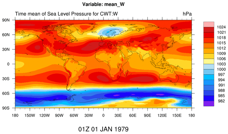
Fig. 2 Mean sea level pressure of circulation weather type West.

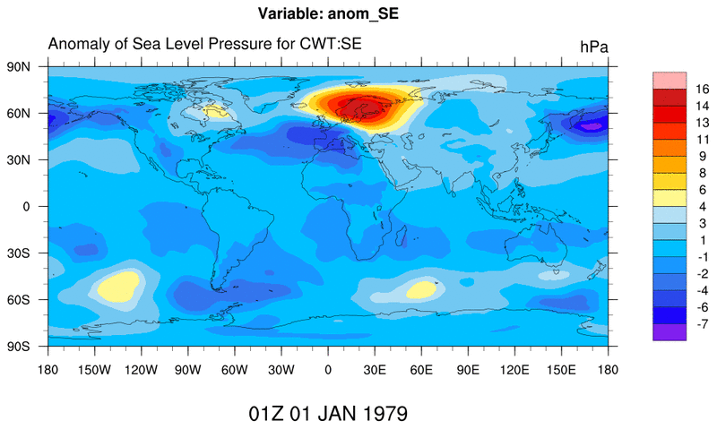
Fig. 3 Anomaly of sea level pressure of circulation weather type West.